Inverse probability weighting and marginal structural models
What If: Chapter 12
Elena Dudukina
2021-04-29
1 / 24
12.1 The causal question
- Average treatment effect (ATE), or average causal effect (ACE) of smoking cessation on weight gain
- Causal contrast to assess: E[Ya=1]−E[Ya=0]
- Marginal weight gain difference had everyone stopped smoking vs had no one stopped smoking (everyone was treated vs everyone was untreated)
- Ignoring loss-to-follow-up from 1971 (baseline) through 1982
- Ignoring time-varying nature of the treatment and potential time-varying confounding
- Assuming conditional exchangeability based on age, sex, race, education, smoking intensity and duration, physical activity, exercise, and baseline weight
2 / 24
library(tidyverse)library(magrittr)# getting the datadata <- readr::read_csv(file = "https://cdn1.sph.harvard.edu/wp-content/uploads/sites/1268/1268/20/nhefs.csv") %>% mutate( education = case_when( education == 1 ~ "8th grade or less", education == 2 ~ "HS dropout", education == 3 ~ "HS", education == 4 ~ "College dropout", education == 5 ~ "College or more", T ~ "missing" ) ) %>% mutate(across(.cols = c(qsmk, sex, race, education, exercise, active), .fns = forcats::as_factor)) %>% drop_na(qsmk, sex, race, education, exercise, active, wt82)# what's inside?data %>% select(qsmk, age, sex, race, education, wt71, smokeintensity, smokeyrs, exercise, active)## # A tibble: 1,566 x 10## qsmk age sex race education wt71 smokeintensity smokeyrs exercise## <fct> <dbl> <fct> <fct> <fct> <dbl> <dbl> <dbl> <fct> ## 1 0 42 0 1 8th grade or ~ 79.0 30 29 2 ## 2 0 36 0 0 HS dropout 58.6 20 24 0 ## 3 0 56 1 1 HS dropout 56.8 20 26 2 ## 4 0 68 0 1 8th grade or ~ 59.4 3 53 2 ## 5 0 40 0 0 HS dropout 87.1 20 19 1 ## 6 0 43 1 1 HS dropout 99 10 21 1 ## 7 0 56 1 0 HS 63.0 20 39 1 ## 8 0 29 1 0 HS 58.7 2 9 2 ## 9 0 51 0 0 HS dropout 64.9 25 37 2 ## 10 0 43 0 0 HS dropout 62.3 20 25 2 ## # ... with 1,556 more rows, and 1 more variable: active <fct>| Characteristics | Smokers | Non-smokers |
|---|---|---|
| age | 46.2 (12.2) | 42.8 (11.8) |
| sex | 183 (45.4%) | 621 (53.4%) |
| race | 36 (8.9%) | 170 (14.6%) |
| College or more | 62 (15.4%) | 115 (9.9%) |
| wt71 | 72.4 (15.6) | 70.3 (15.2) |
| smokeintensity | 18.6 (12.4) | 21.2 (11.5) |
| smokeyrs | 26.0 (12.7) | 24.1 (11.7) |
| exercise | 164 (40.7%) | 441 (37.9%) |
| active | 45 (11.2%) | 104 (8.9%) |
3 / 24
12.1 The causal question
- What is the average causal effect of smoking cessation on body weight gain?
- Crude associational estimate
- ˆE[Y|A=1] - ˆE[Y|A=0]
- Does not have a causal interpretation because exchangeability does not hold
- Quitters and non-quitters are different in respect to characteristics affecting weight gain
data %>% group_by(qsmk) %>% summarise("Mean weight difference with baseline, kg" = mean(wt82_71))## # A tibble: 2 x 2## qsmk `Mean weight difference with baseline, kg`## <fct> <dbl>## 1 0 1.98## 2 1 4.53lm(data = data, formula = wt82_71 ~ qsmk) %>% broom::tidy(., conf.int = T) %>% select(term, conf.low, estimate, conf.high)## # A tibble: 2 x 4## term conf.low estimate conf.high## <chr> <dbl> <dbl> <dbl>## 1 (Intercept) 1.54 1.98 2.43## 2 qsmk1 1.66 2.54 3.434 / 24
Causal asumptions recap: exchangeability
- Exchangeability: Ya⊥⊥ A
- Treated individuals (A=1) had they been untreated (A=0) had the same probability of the potential outcome (PO)
- Conditional exchangeability: Ya⊥⊥ A|L, where L closes all back-door paths between A and Y
- When accounted for all variables in L, treated individuals (A=1) had they been untreated (A=0) had the same probability of the potential outcome
- Confounding is a lack of exchangeability
- Confounders are variables, which when adjusted for, restore exchangeability, or remove confounding
- Untestable
5 / 24
Causal asumptions recap: positivity
- Positive probability of observing each level of treatment in each strata of L
- Pr(A=a|L=l>0) for all a and l
- Only relevant for variables L required for exchangeability
- Can be empirically verified
6 / 24
Causal asumptions recap: consistency
- We observe PO - the one under actually received treatment
- Pr[Ya=1|A=1]=Pr[Y=1|A=1]
- Well-defined intervention paradigm: treatment as several versions of the intervention
- Are all versions observed and measured?
- Do all versions of the treatment have the same causal effect?
- Not well-defined values of a lead to not well-defined PO Ya under the levels of treatment and the causal contrast Pr[Ya=1=1]−Pr[Ya=0=1] is not well-defined
- When dealing with treatments with multiple versions ➡️ assuming treatment variation irrelevance
- More details on causal assumptions in Chapter 3
7 / 24
12.1 The causal question
- Quitters and non-quitters differ in a variety of ways
- L is vector variable:
- age
- sex
- race
- education
- smoking intensity
- smoking duration
- physical activity
- exercise
- baseline weight
- Ya⊥⊥ A|L
- Adjustment (standardization) formula: El[Y|A=a,L=l]Pr[L=l]
8 / 24
12.2 Estimating IPT weights via modeling
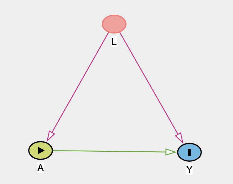
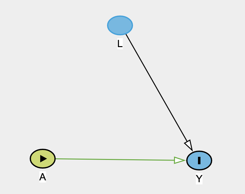
- IPTW ➡️ pseudo-population in which the arrow from L to the treatment A is removed
- A⊥⊥ L
- Eps[Y|A=a] = El[Y|A=a,L=l]Pr[L=l]
- Mean outcome expectation in the IPT-weighted population equals the standardized mean outcome in the initial population
- If Ya⊥⊥ A|L holds in the initial population:
- Mean PO Ya is the same in initial and IPT-weighted populations
- Marginal (unconditional exchangeability) holds in the IPT-weighted population
- Counterfactual mean E[Ya] in the initial population equals observed mean in IPT-weighted population Eps[Y|A=a]
- In the IPT-weighted population observed associational quantity has a causal interpretation
- Initial population

- IPT-weighted population

9 / 24
12.2 Estimating IPT weights via modeling
- Denominator: Pr[A=1|L] in treated and Pr[A=0|L] in untreated, i.e. 1−Pr[A=1|L]
- Numerator:
- Non-stabilized: 1
- Stabilized: Pr[A=1]
- Stabilized weights usually give narrower 95% confidence intervals than nonstabilized weights
- In the example code: GEE models with an independent working correlation for 95% CIs
- I will use bootstrap
10 / 24
- Code IPTW
- IPTW distribution code
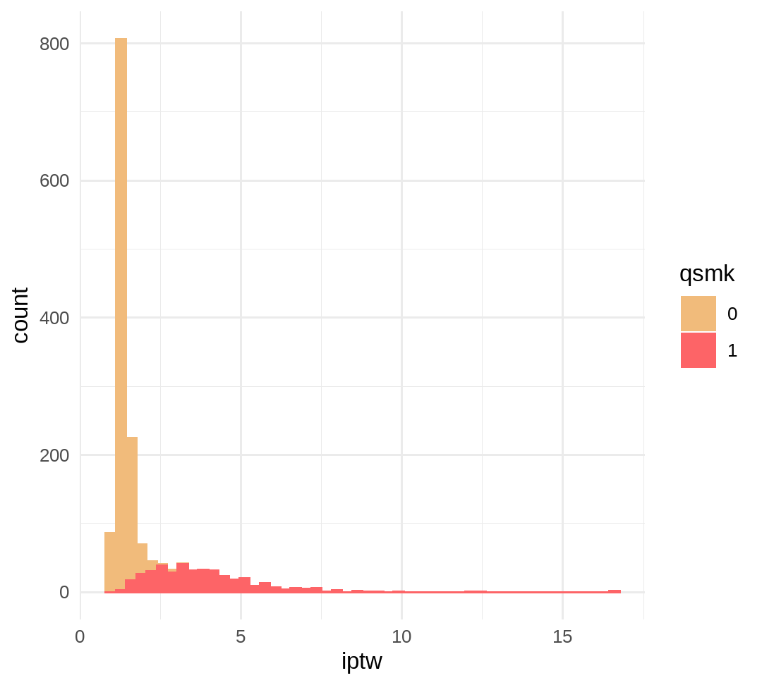
- IPTW distribution unstab
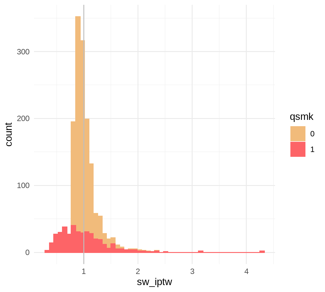
- IPTW distribution stab
- results code
- 95% CIs bootstrap for stab weights
- 95% CIs bootstrap for unstab weights
pr_a <- glm(data = data, formula = qsmk~1, family = binomial("logit"))pr_a_l <- glm(data = data, formula = qsmk ~ sex + race + age + I(age*age) + education + smokeintensity + I(smokeintensity*smokeintensity) + smokeyrs + I(smokeyrs*smokeyrs) + exercise + active + wt71 + I(wt71*wt71), family = binomial("logit"))data %<>% mutate( p_a = predict(object = pr_a, type = "response"), p_a_l = predict(object = pr_a_l, type = "response"), # for average treatment effect iptw = if_else(qsmk == 1, 1/p_a_l, 1/(1-p_a_l)), # unstabilized weights sw_iptw = if_else(qsmk == 1, p_a/p_a_l, (1-p_a)/(1-p_a_l)) # stabilized weights)p_iptw <- data %>% group_by(qsmk) %>% ggplot(aes(x = iptw, color = qsmk, fill = qsmk)) + geom_histogram(bins = 50) + theme_minimal() + scale_fill_manual(values = wesanderson::wes_palette("GrandBudapest1", n = 2)) + scale_color_manual(values = wesanderson::wes_palette("GrandBudapest1", n = 2))p_sw_iptw <- data %>% group_by(qsmk) %>% ggplot(aes(x = sw_iptw, color = qsmk, fill = qsmk)) + geom_histogram(bins = 50) + theme_minimal() + scale_fill_manual(values = wesanderson::wes_palette("GrandBudapest1", n = 2)) + scale_color_manual(values = wesanderson::wes_palette("GrandBudapest1", n = 2)) + geom_vline(xintercept = 1, color = "grey")# expected mean=2summary(data$iptw)## Min. 1st Qu. Median Mean 3rd Qu. Max. ## 1.054 1.230 1.373 1.996 1.990 16.700p_iptw
# expected mean=1summary(data$sw_iptw)## Min. 1st Qu. Median Mean 3rd Qu. Max. ## 0.3312 0.8665 0.9503 0.9988 1.0793 4.2977p_sw_iptw
# 95% CIs are incorrectglm(data = data, formula = wt82_71~qsmk, family = gaussian(), weights = iptw) %>% broom::tidy(., conf.int = T) %>% select(term, conf.low, estimate, conf.high)## # A tibble: 2 x 4## term conf.low estimate conf.high## <chr> <dbl> <dbl> <dbl>## 1 (Intercept) 1.22 1.78 2.34## 2 qsmk1 2.64 3.44 4.24glm(data = data, formula = wt82_71~qsmk, family = gaussian(), weights = sw_iptw) %>% broom::tidy(., conf.int = T) %>% select(term, conf.low, estimate, conf.high)## # A tibble: 2 x 4## term conf.low estimate conf.high## <chr> <dbl> <dbl> <dbl>## 1 (Intercept) 1.33 1.78 2.23## 2 qsmk1 2.56 3.44 4.32library(tidymodels)set.seed(972188635)boots <- bootstraps(data, times = 1e3, apparent = FALSE)iptw_model_sw <- function(data) { glm(formula = wt82_71 ~ qsmk, family = gaussian(), weight = sw_iptw, data = data)}boot_models <- boots %>% mutate( model = map(.x = splits, ~iptw_model_sw(data = .x)), coef_info = map(model, ~broom::tidy(.x)))int_pctl(boot_models, coef_info) # M. Hernan: 3.4 (2.4-4.5)## # A tibble: 2 x 6## term .lower .estimate .upper .alpha .method ## <chr> <dbl> <dbl> <dbl> <dbl> <chr> ## 1 (Intercept) 1.32 1.78 2.21 0.05 percentile## 2 qsmk1 2.42 3.44 4.48 0.05 percentileint_pctl(.data = boot_models_unst, statistics = coef_info)## # A tibble: 2 x 6## term .lower .estimate .upper .alpha .method ## <chr> <dbl> <dbl> <dbl> <dbl> <chr> ## 1 (Intercept) 1.32 1.78 2.21 0.05 percentile## 2 qsmk1 2.42 3.44 4.48 0.05 percentile11 / 24
12.2 IPT-unweighted and weighted populations
data %>% group_by(qsmk) %>% count(education) %>% mutate(pct = n/sum(n)*100)## # A tibble: 10 x 4## # Groups: qsmk [2]## qsmk education n pct## <fct> <fct> <int> <dbl>## 1 0 8th grade or less 210 18.1 ## 2 0 HS dropout 266 22.9 ## 3 0 HS 480 41.3 ## 4 0 College or more 115 9.89## 5 0 College dropout 92 7.91## 6 1 8th grade or less 81 20.1 ## 7 1 HS dropout 74 18.4 ## 8 1 HS 157 39.0 ## 9 1 College or more 62 15.4 ## 10 1 College dropout 29 7.20data %>% group_by(qsmk) %>% count(education, wt = sw_iptw) %>% mutate(pct = n/sum(n)*100)## # A tibble: 10 x 4## # Groups: qsmk [2]## qsmk education n pct## <fct> <fct> <dbl> <dbl>## 1 0 8th grade or less 214. 18.4 ## 2 0 HS dropout 253. 21.7 ## 3 0 HS 472. 40.6 ## 4 0 College or more 134. 11.5 ## 5 0 College dropout 89.7 7.72## 6 1 8th grade or less 69.8 17.4 ## 7 1 HS dropout 87.8 21.8 ## 8 1 HS 164. 40.8 ## 9 1 College or more 46.4 11.5 ## 10 1 College dropout 33.8 8.4112 / 24
Fine Point 12.2: Checking positivity
- Structural violations
- Individuals with some levels of confounders cannot be treated (contraindcations for medications, etc.)
- Causal inferences are impossible for the entire population using IPW or standardization
- Random violations
- Finite data sample
- Parametric modeling to smooth over random zeroes
13 / 24
12.4 Marginal structural models (MSMs)
- Models for marginal potential outcomes
- Marginal: marginal effect of exposure on the outcome
- Structural: for PO
- Marginal structural mean model for the smoking example:
- E[Ya]=β0+β1a
- We estimated parameter β1 of MSM 👆, or ATE of smoking cessation if all were quitters vs non-quitters E[Ya=1]−E[Ya=0] Given causal assumptions:
- E[Ya=1]−E[Ya=0]
- = E[Ya=1|L]−E[Ya=0|L] : under law of total probability
- = E[Ya=1|L,A=1]−E[Ya=0|L,A=0] : under conditional echangeability Ya⊥⊥A|L
- = E[Y|L,A=1]−E[Y|L,A=0] : under consistency
14 / 24
12.4 Marginal structural models (MSMs)
- Effect of ⬆️ smoking intensity by 20 cigarettes per day compared with no change?
- Estimate parameters of MSM: E[Ya=20]=β0+β1∗20+β2∗400 ➡️ E[Ya=20]−E[Ya=0]; β1, β2?
- Hernan: β0=2.005, β1 = -0.109, β2 = 0.003
data_smkint <- data %>% filter(smokeintensity < 26)data_smkint## # A tibble: 1,162 x 68## seqn qsmk death yrdth modth dadth sbp dbp sex age race income## <dbl> <fct> <dbl> <dbl> <dbl> <dbl> <dbl> <dbl> <fct> <dbl> <fct> <dbl>## 1 235 0 0 NA NA NA 123 80 0 36 0 18## 2 244 0 0 NA NA NA 115 75 1 56 1 15## 3 245 0 1 85 2 14 148 78 0 68 1 15## 4 252 0 0 NA NA NA 118 77 0 40 0 18## 5 257 0 0 NA NA NA 141 83 1 43 1 11## 6 262 0 0 NA NA NA 132 69 1 56 0 19## 7 266 0 0 NA NA NA 100 53 1 29 0 22## 8 419 0 1 84 10 13 163 79 0 51 0 18## 9 420 0 1 86 10 17 184 106 0 43 0 16## 10 434 0 0 NA NA NA 127 80 1 54 0 16## # ... with 1,152 more rows, and 56 more variables: marital <dbl>, school <dbl>,## # education <fct>, ht <dbl>, wt71 <dbl>, wt82 <dbl>, wt82_71 <dbl>,## # birthplace <dbl>, smokeintensity <dbl>, smkintensity82_71 <dbl>,## # smokeyrs <dbl>, asthma <dbl>, bronch <dbl>, tb <dbl>, hf <dbl>, hbp <dbl>,## # pepticulcer <dbl>, colitis <dbl>, hepatitis <dbl>, chroniccough <dbl>,## # hayfever <dbl>, diabetes <dbl>, polio <dbl>, tumor <dbl>,## # nervousbreak <dbl>, alcoholpy <dbl>, alcoholfreq <dbl>, alcoholtype <dbl>,## # alcoholhowmuch <dbl>, pica <dbl>, headache <dbl>, otherpain <dbl>,## # weakheart <dbl>, allergies <dbl>, nerves <dbl>, lackpep <dbl>,## # hbpmed <dbl>, boweltrouble <dbl>, wtloss <dbl>, infection <dbl>,## # active <fct>, exercise <fct>, birthcontrol <dbl>, pregnancies <dbl>,## # cholesterol <dbl>, hightax82 <dbl>, price71 <dbl>, price82 <dbl>,## # tax71 <dbl>, tax82 <dbl>, price71_82 <dbl>, tax71_82 <dbl>, p_a <dbl>,## # p_a_l <dbl>, iptw <dbl>, sw_iptw <dbl>15 / 24
IPTW for smkintensity82_71
pr_a <- lm(data = data_smkint, formula = smkintensity82_71~1)pr_a_l <- lm(data = data_smkint, formula = smkintensity82_71 ~ sex + race + age + I(age*age) + education + smokeintensity + I(smokeintensity*smokeintensity) + smokeyrs + I(smokeyrs*smokeyrs) + exercise + active + wt71 + I(wt71*wt71))sd_a <- summary(pr_a)$sigmasd_a_l <- summary(pr_a_l)$sigmadata_smkint %<>% mutate( p_a = predict(object = pr_a, type = "response"), p_a_l = predict(object = pr_a_l, type = "response"), density_num = dnorm(x = smkintensity82_71, mean = p_a, sd = sd_a), density_denom = dnorm(x = smkintensity82_71, mean = p_a_l, sd = sd_a_l), # for average treatment effect sw_iptw = density_num/density_denom)summary(data_smkint$sw_iptw)## Min. 1st Qu. Median Mean 3rd Qu. Max. ## 0.1938 0.8872 0.9710 0.9968 1.0545 5.1023set.seed(198877)boots <- bootstraps(data_smkint, times = 1e3, apparent = FALSE)iptw_model <- function(data) { glm(formula = wt82_71 ~ smkintensity82_71 + I(smkintensity82_71*smkintensity82_71), family = gaussian(), weight = sw_iptw, data = data)}boot_models <- boots %>% mutate( model = map(.x = splits, ~iptw_model(data = .x)), coef_info = map(model, ~broom::tidy(.x)))int_pctl(.data = boot_models, statistics = coef_info)## # A tibble: 3 x 6## term .lower .estimate .upper .alpha .method ## <chr> <dbl> <dbl> <dbl> <dbl> <chr> ## 1 (Intercept) 1.38 1.98 2.51 0.05 percenti~## 2 I(smkintensity82_71 * smkintens~ -0.000884 0.00317 0.00900 0.05 percenti~## 3 smkintensity82_71 -0.164 -0.106 -0.0444 0.05 percenti~16 / 24
12.4 Marginal structural models (MSMs)
- Dichotomous outcome: death
- MSM: logit Pr[Da=1]=α0+α1a
- Hernan: 1.0 (0.8, 1.4)
17 / 24
12.4 MSMs
pr_a <- glm(data = data, formula = qsmk~1, family = binomial("logit"))pr_a_l <- glm(data = data, formula = qsmk ~ sex + race + age + I(age*age) + education + smokeintensity + I(smokeintensity*smokeintensity) + smokeyrs + I(smokeyrs*smokeyrs) + exercise + active + wt71 + I(wt71*wt71), family = binomial("logit"))data %<>% mutate( p_a = predict(object = pr_a, type = "response"), p_a_l = predict(object = pr_a_l, type = "response"), sw_iptw = if_else(qsmk == 1, p_a/p_a_l, (1-p_a)/(1-p_a_l)) # stabilized weights)set.seed(198877)boots <- bootstraps(data, times = 1e3, apparent = FALSE)iptw_model_death <- function(data) { glm(formula = death ~ qsmk, family = binomial(link = "logit"), weight = sw_iptw, data = data)}boot_models <- boots %>% mutate( model = map(.x = splits, ~iptw_model_death(data = .x)), coef_info = map(model, ~broom::tidy(.x, exponentiate = T)))int_pctl(.data = boot_models, statistics = coef_info)## # A tibble: 2 x 6## term .lower .estimate .upper .alpha .method ## <chr> <dbl> <dbl> <dbl> <dbl> <chr> ## 1 (Intercept) 0.191 0.225 0.262 0.05 percentile## 2 qsmk1 0.732 1.04 1.39 0.05 percentile18 / 24
12.5 Effect modification and marginal structural models
- Stratification by a true effect measure modifiers (EMM) (not confounders)
- EMM by sex:
- E[Ya|sex]=β0+β1a+β2a∗sex+β3∗sex
- The model is now marginal over confounders L, but conditional on sex
- IPTW: Pr[A|sex]Pr[A|L]
- Hernan: 95% CI for estimate of β2 parameter (-2.2; 1.9)
19 / 24
12.5 Effect modification and marginal structural models
pr_a <- glm(data = data, formula = qsmk~sex, family = binomial("logit"))pr_a_l <- glm(data = data, formula = qsmk ~ sex + race + age + I(age*age) + education + smokeintensity + I(smokeintensity*smokeintensity) + smokeyrs + I(smokeyrs*smokeyrs) + exercise + active + wt71 + I(wt71*wt71), family = binomial("logit"))data %<>% mutate( p_a = predict(object = pr_a, type = "response"), p_a_l = predict(object = pr_a_l, type = "response"), sw_iptw = if_else(qsmk == 1, p_a/p_a_l, (1-p_a)/(1-p_a_l)) # stabilized weights)set.seed(972188635)boots <- bootstraps(data, times = 1e3, apparent = FALSE)iptw_model_sw <- function(data) { glm(formula = wt82_71 ~ qsmk*sex, family = gaussian(), weight = sw_iptw, data = data)}boot_models <- boots %>% mutate( model = map(.x = splits, ~iptw_model_sw(data = .x)), coef_info = map(model, ~broom::tidy(.x)))int_pctl(boot_models, coef_info)## # A tibble: 4 x 6## term .lower .estimate .upper .alpha .method ## <chr> <dbl> <dbl> <dbl> <dbl> <chr> ## 1 (Intercept) 1.19 1.79 2.41 0.05 percentile## 2 qsmk1 2.11 3.52 4.81 0.05 percentile## 3 qsmk1:sex1 -2.08 -0.143 1.94 0.05 percentile## 4 sex1 -0.943 -0.0286 0.829 0.05 percentile20 / 24
12.6 Censoring and missing data
Unstabilized IPCW 1Pr[C=0|A,L] create a pseudo-population before censoring (no selection and no selection bias)
Stabilized IPCW Pr[C=0|A]Pr[C=0|A,L] essentially create a pseudo-population, in which instead of informative censoring, there's censoring at random (there is selection, but no selection bias)
Joint treatment (A, C)
Joint identifiability assumptions:
- Joint exchangeability Ya,c=0⊥⊥(A,C)|L
- Joint positivity
- Joint consistency
3.5 kg (95% confidence interval: 2.5, 4.5)
21 / 24
12.6 Censoring and missing data
data <- readr::read_csv(file = "https://cdn1.sph.harvard.edu/wp-content/uploads/sites/1268/1268/20/nhefs.csv") %>% mutate( education = case_when( education == 1 ~ "8th grade or less", education == 2 ~ "HS dropout", education == 3 ~ "HS", education == 4 ~ "College dropout", education == 5 ~ "College or more", T ~ "missing" ), cens = case_when( is.na(wt82) ~ 1, T ~ 0 ) ) %>% mutate(across(.cols = c(qsmk, sex, race, education, exercise, active, cens), .fns = forcats::as_factor))22 / 24
12.6 Censoring and missing data
- Addressing loss-to-follow-up
| Characteristics | Non-smokers | Smokers |
|---|---|---|
| n = 1566 | n = 63 | |
| cens | ||
| 0 | 1566 (100%) | 0 (0%) |
| 1 | 0 (0%) | 63 (100%) |
| qsmk | ||
| 0 | 1163 (74.3%) | 38 (60.3%) |
| 1 | 403 (25.7%) | 25 (39.7%) |
| wt71 | ||
| 70.8 (15.3) | 76.6 (23.3) |
pr_a <- glm(data = data, formula = qsmk~1, family = binomial("logit"))pr_a_l <- glm(data = data, formula = qsmk ~ sex + race + age + I(age*age) + education + smokeintensity + I(smokeintensity*smokeintensity) + smokeyrs + I(smokeyrs*smokeyrs) + exercise + active + wt71 + I(wt71*wt71), family = binomial("logit"))data %<>% mutate( p_a = predict(object = pr_a, type = "response"), p_a_l = predict(object = pr_a_l, type = "response"), sw_iptw = if_else(qsmk == 1, p_a/p_a_l, (1-p_a)/(1-p_a_l)) # stabilized weights)pr_c <- glm(data = data, formula = cens~qsmk, family = binomial("logit"))pr_c_l <- glm(data = data, formula = cens ~ qsmk + sex + race + age + I(age*age) + education + smokeintensity + I(smokeintensity*smokeintensity) + smokeyrs + I(smokeyrs*smokeyrs) + exercise + active + wt71 + I(wt71*wt71), family = binomial("logit"))data %<>% mutate( p_c = predict(object = pr_c, type = "response"), p_c_l = predict(object = pr_c_l, type = "response"), sw_ipcw = if_else(cens == 0, (1-p_c)/(1-p_c_l), 1), w = sw_iptw * sw_ipcw)summary(data$sw_iptw)## Min. 1st Qu. Median Mean 3rd Qu. Max. ## 0.3312 0.8640 0.9504 0.9991 1.0755 4.2054summary(data$sw_ipcw)## Min. 1st Qu. Median Mean 3rd Qu. Max. ## 0.9442 0.9785 0.9868 0.9991 1.0022 1.7180summary(data$w)## Min. 1st Qu. Median Mean 3rd Qu. Max. ## 0.3546 0.8567 0.9448 0.9978 1.0737 4.0931set.seed(9721835)boots <- bootstraps(data, times = 1e3, apparent = FALSE)w_model <- function(data) { glm(formula = wt82_71 ~ qsmk, family = gaussian(), weight = w, data = data)}boot_models <- boots %>% mutate( model = map(.x = splits, ~w_model(data = .x)), coef_info = map(model, ~broom::tidy(.x)))int_pctl(boot_models, coef_info)## # A tibble: 2 x 6## term .lower .estimate .upper .alpha .method ## <chr> <dbl> <dbl> <dbl> <dbl> <chr> ## 1 (Intercept) 1.21 1.67 2.11 0.05 percentile## 2 qsmk1 2.49 3.47 4.49 0.05 percentile23 / 24
References
Hernán MA, Robins JM (2020). Causal Inference: What If. Boca Raton: Chapman & Hall/CRC (v. 30mar21)
24 / 24