Inverse probability weighting and marginal structural modelsWhat If: Chapter 12Elena Dudukina2021-04-291 / 24

12.1 The causal questionAverage treatment effect (ATE), or average causal effect (ACE) of smoking cessation on weight gain
Causal contrast to assess: E[Ya=1]−E[Ya=0]E[Ya=1]−E[Ya=0]
Marginal weight gain difference had everyone stopped smoking vs had no one stopped smoking (everyone was treated vs everyone was untreated)
Ignoring loss-to-follow-up from 1971 (baseline) through 1982
Ignoring time-varying nature of the treatment and potential time-varying confounding
Assuming conditional exchangeability based on age, sex, race, education, smoking intensity and duration, physical activity, exercise, and baseline weight
2 / 24

Code
Data
Table 12.1
library(tidyverse)
library(magrittr)
# getting the data
data <- readr::read_csv(file = "https://cdn1.sph.harvard.edu/wp-content/uploads/sites/1268/1268/20/nhefs.csv") %>% 
  mutate(
    education = case_when(
      education == 1  ~ "8th grade or less",
      education == 2 ~ "HS dropout",
      education == 3 ~ "HS",
      education == 4 ~ "College dropout",
      education == 5 ~ "College or more",
      T ~ "missing"
    )
  ) %>% 
  mutate(across(.cols = c(qsmk, sex, race, education, exercise, active), .fns = forcats::as_factor)) %>% 
  drop_na(qsmk, sex, race, education, exercise, active, wt82)
# what's inside?
data %>% select(qsmk, age, sex, race, education, wt71, smokeintensity, smokeyrs, exercise, active)
## # A tibble: 1,566 x 10
##    qsmk    age sex   race  education       wt71 smokeintensity smokeyrs exercise
##    <fct> <dbl> <fct> <fct> <fct>          <dbl>          <dbl>    <dbl> <fct>   
##  1 0        42 0     1     8th grade or ~  79.0             30       29 2       
##  2 0        36 0     0     HS dropout      58.6             20       24 0       
##  3 0        56 1     1     HS dropout      56.8             20       26 2       
##  4 0        68 0     1     8th grade or ~  59.4              3       53 2       
##  5 0        40 0     0     HS dropout      87.1             20       19 1       
##  6 0        43 1     1     HS dropout      99               10       21 1       
##  7 0        56 1     0     HS              63.0             20       39 1       
##  8 0        29 1     0     HS              58.7              2        9 2       
##  9 0        51 0     0     HS dropout      64.9             25       37 2       
## 10 0        43 0     0     HS dropout      62.3             20       25 2       
## # ... with 1,556 more rows, and 1 more variable: active <fct>

 
    Characteristics 
    Smokers 
    Non-smokers 
  


    age 
    46.2 (12.2) 
    42.8 (11.8) 
  

    sex 
    183 (45.4%) 
    621 (53.4%) 
  

    race 
    36 (8.9%) 
    170 (14.6%) 
  

    College or more 
    62 (15.4%) 
    115 (9.9%) 
  

    wt71 
    72.4 (15.6) 
    70.3 (15.2) 
  

    smokeintensity 
    18.6 (12.4) 
    21.2 (11.5) 
  

    smokeyrs 
    26.0 (12.7) 
    24.1 (11.7) 
  

    exercise 
    164 (40.7%) 
    441 (37.9%) 
  

    active 
    45 (11.2%) 
    104 (8.9%) 
  

3 / 24

Characteristics	Smokers	Non-smokers
age	46.2 (12.2)	42.8 (11.8)
sex	183 (45.4%)	621 (53.4%)
race	36 (8.9%)	170 (14.6%)
College or more	62 (15.4%)	115 (9.9%)
wt71	72.4 (15.6)	70.3 (15.2)
smokeintensity	18.6 (12.4)	21.2 (11.5)
smokeyrs	26.0 (12.7)	24.1 (11.7)
exercise	164 (40.7%)	441 (37.9%)
active	45 (11.2%)	104 (8.9%)

12.1 The causal question

What is the average causal effect of smoking cessation on body weight gain?
Crude associational estimate
$\hat{E} [Y | A = 1]$ - $\hat{E} [Y | A = 0]$
Does not have a causal interpretation because exchangeability does not hold
- Quitters and non-quitters are different in respect to characteristics affecting weight gain

data %>% 
  group_by(qsmk) %>% 
  summarise("Mean weight difference with baseline, kg" = mean(wt82_71))

## # A tibble: 2 x 2
##   qsmk  `Mean weight difference with baseline, kg`
##   <fct>                                      <dbl>
## 1 0                                           1.98
## 2 1                                           4.53

lm(data = data, formula = wt82_71 ~ qsmk) %>% broom::tidy(., conf.int = T) %>% select(term, conf.low, estimate, conf.high)

## # A tibble: 2 x 4
##   term        conf.low estimate conf.high
##   <chr>          <dbl>    <dbl>     <dbl>
## 1 (Intercept)     1.54     1.98      2.43
## 2 qsmk1           1.66     2.54      3.43

4 / 24

Causal asumptions recap: exchangeabilityExchangeability: Ya⊥⊥ AYa⊥⊥ A
Treated individuals (A=1) had they been untreated (A=0) had the same probability of the potential outcome (PO)Conditional exchangeability: Ya⊥⊥ A|LYa⊥⊥ A|L, where L closes all back-door paths between A and Y
When accounted for all variables in L, treated individuals (A=1) had they been untreated (A=0) had the same probability of the potential outcome

Confounding is a lack of exchangeability
Confounders are variables, which when adjusted for, restore exchangeability, or remove confounding
Untestable
5 / 24

Causal asumptions recap: positivityPositive probability of observing each level of treatment in each strata of L
Pr(A=a|L=l>0)Pr(A=a|L=l>0) for all aa and ll
Only relevant for variables L required for exchangeability
Can be empirically verified
6 / 24

Causal asumptions recap: consistencyWe observe PO - the one under actually received treatmentPr[Ya=1|A=1]=Pr[Y=1|A=1]Pr[Ya=1|A=1]=Pr[Y=1|A=1]

Well-defined intervention paradigm: treatment as several versions of the interventionAre all versions observed and measured?
Do all versions of the treatment have the same causal effect?
Not well-defined values of aa lead to not well-defined PO YaYa under the levels of treatment and the causal contrast Pr[Ya=1=1]−Pr[Ya=0=1]Pr[Ya=1=1]−Pr[Ya=0=1] is not well-defined
When dealing with treatments with multiple versions ➡️ assuming treatment variation irrelevance

More details on causal assumptions in Chapter 3
7 / 24

12.1 The causal questionQuitters and non-quitters differ in a variety of ways
L is vector variable:age
sex
race
education
smoking intensity
smoking duration
physical activity
exercise
baseline weight

Ya⊥⊥ A|LYa⊥⊥ A|L
Adjustment (standardization) formula: El[Y|A=a,L=l]Pr[L=l]El[Y|A=a,L=l]Pr[L=l]
8 / 24

12.2 Estimating IPT weights via modeling

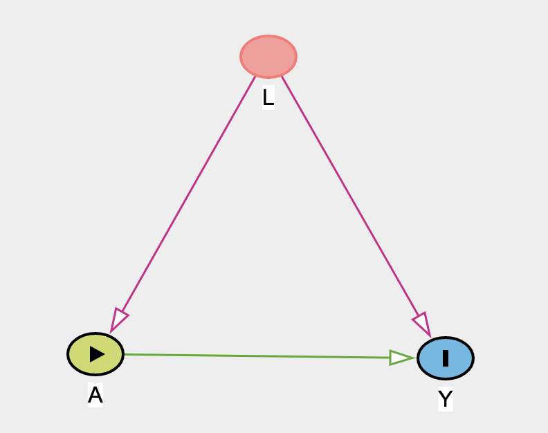
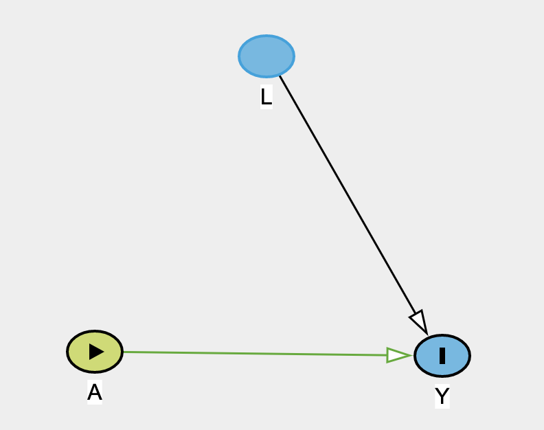
IPTW ➡️ pseudo-population in which the arrow from L to the treatment A is removed
- $A ⊥⊥ L$
- $E_{p s} [Y | A = a]$ = $E_{l} [Y | A = a, L = l] P r [L = l]$
  - Mean outcome expectation in the IPT-weighted population equals the standardized mean outcome in the initial population
If $Y^{a} ⊥⊥ A | L$ holds in the initial population:
- Mean PO $Y^{a}$ is the same in initial and IPT-weighted populations
- Marginal (unconditional exchangeability) holds in the IPT-weighted population
- Counterfactual mean $E [Y^{a}]$ in the initial population equals observed mean in IPT-weighted population $E_{p s} [Y | A = a]$
- In the IPT-weighted population observed associational quantity has a causal interpretation

Initial population

IPT-weighted population

9 / 24

12.2 Estimating IPT weights via modelingDenominator: Pr[A=1|L]Pr[A=1|L] in treated and Pr[A=0|L]Pr[A=0|L] in untreated, i.e. 1−Pr[A=1|L]1−Pr[A=1|L]
Numerator:Non-stabilized: 1
Stabilized: Pr[A=1]Pr[A=1]

Stabilized weights usually give narrower 95% confidence intervals than nonstabilized weights
In the example code: GEE models with an independent working correlation for 95% CIs
I will use bootstrap
10 / 24

pr_a <- glm(data = data, formula = qsmk~1, family = binomial("logit"))
pr_a_l <- glm(data = data, formula = qsmk ~ sex + race + age + I(age*age) + education + smokeintensity + I(smokeintensity*smokeintensity) + smokeyrs + I(smokeyrs*smokeyrs) + exercise + active + wt71 + I(wt71*wt71), family = binomial("logit"))
data %<>% mutate(
  p_a = predict(object = pr_a, type = "response"),
  p_a_l = predict(object = pr_a_l, type = "response"),
  # for average treatment effect
  iptw = if_else(qsmk == 1, 1/p_a_l, 1/(1-p_a_l)), # unstabilized weights
  sw_iptw = if_else(qsmk == 1, p_a/p_a_l, (1-p_a)/(1-p_a_l)) # stabilized weights
)

p_iptw <- data %>% 
  group_by(qsmk) %>% 
  ggplot(aes(x = iptw, color = qsmk, fill = qsmk)) +
  geom_histogram(bins = 50) +
  theme_minimal() +
  scale_fill_manual(values = wesanderson::wes_palette("GrandBudapest1", n = 2)) +
  scale_color_manual(values = wesanderson::wes_palette("GrandBudapest1", n = 2))
p_sw_iptw <- data %>% 
  group_by(qsmk) %>% 
  ggplot(aes(x = sw_iptw, color = qsmk, fill = qsmk)) +
  geom_histogram(bins = 50) +
  theme_minimal() +
  scale_fill_manual(values = wesanderson::wes_palette("GrandBudapest1", n = 2)) +
  scale_color_manual(values = wesanderson::wes_palette("GrandBudapest1", n = 2)) +
  geom_vline(xintercept = 1, color = "grey")

# expected mean=2
summary(data$iptw)

##    Min. 1st Qu.  Median    Mean 3rd Qu.    Max. 
##   1.054   1.230   1.373   1.996   1.990  16.700

p_iptw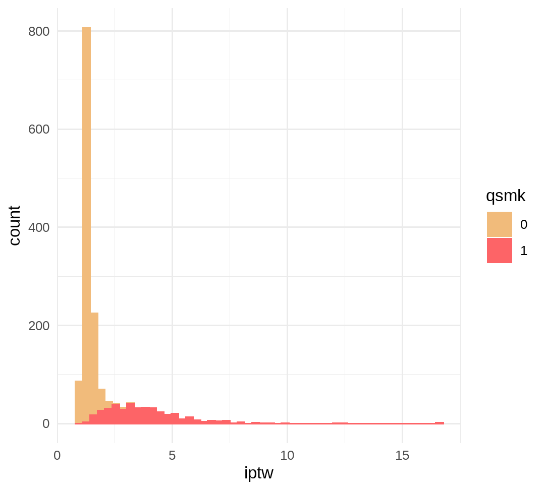

# expected mean=1
summary(data$sw_iptw)

##    Min. 1st Qu.  Median    Mean 3rd Qu.    Max. 
##  0.3312  0.8665  0.9503  0.9988  1.0793  4.2977

p_sw_iptw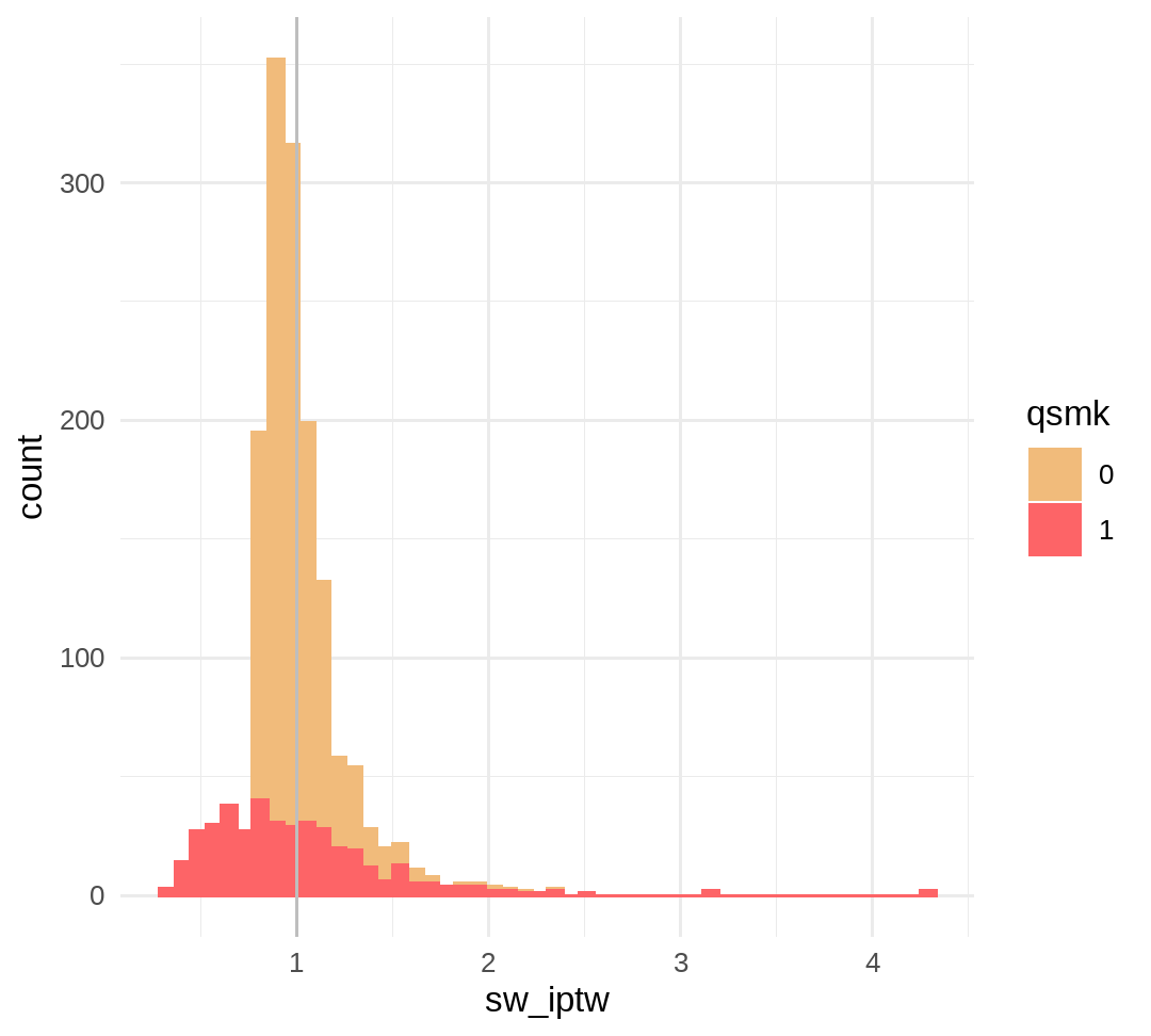

# 95% CIs are incorrect
glm(data = data, formula = wt82_71~qsmk, family = gaussian(), weights = iptw) %>% 
  broom::tidy(., conf.int = T) %>% 
  select(term, conf.low, estimate, conf.high)

## # A tibble: 2 x 4
##   term        conf.low estimate conf.high
##   <chr>          <dbl>    <dbl>     <dbl>
## 1 (Intercept)     1.22     1.78      2.34
## 2 qsmk1           2.64     3.44      4.24

glm(data = data, formula = wt82_71~qsmk, family = gaussian(), weights = sw_iptw) %>% 
  broom::tidy(., conf.int = T) %>% 
  select(term, conf.low, estimate, conf.high)

## # A tibble: 2 x 4
##   term        conf.low estimate conf.high
##   <chr>          <dbl>    <dbl>     <dbl>
## 1 (Intercept)     1.33     1.78      2.23
## 2 qsmk1           2.56     3.44      4.32

library(tidymodels)
set.seed(972188635)
boots <- bootstraps(data, times = 1e3, apparent = FALSE)
iptw_model_sw <- function(data) {
  glm(formula = wt82_71 ~ qsmk, family = gaussian(), weight = sw_iptw, data = data)
}
boot_models <- boots %>% 
  mutate(
    model = map(.x = splits, ~iptw_model_sw(data = .x)),
    coef_info = map(model, ~broom::tidy(.x)))
int_pctl(boot_models, coef_info) # M. Hernan: 3.4 (2.4-4.5)

## # A tibble: 2 x 6
##   term        .lower .estimate .upper .alpha .method   
##   <chr>        <dbl>     <dbl>  <dbl>  <dbl> <chr>     
## 1 (Intercept)   1.32      1.78   2.21   0.05 percentile
## 2 qsmk1         2.42      3.44   4.48   0.05 percentile

int_pctl(.data = boot_models_unst, statistics = coef_info)

## # A tibble: 2 x 6
##   term        .lower .estimate .upper .alpha .method   
##   <chr>        <dbl>     <dbl>  <dbl>  <dbl> <chr>     
## 1 (Intercept)   1.32      1.78   2.21   0.05 percentile
## 2 qsmk1         2.42      3.44   4.48   0.05 percentile

11 / 24

12.2 IPT-unweighted and weighted populationsdata %>% 
  group_by(qsmk) %>% 
  count(education) %>% 
  mutate(pct = n/sum(n)*100)

## # A tibble: 10 x 4
## # Groups:   qsmk [2]
##    qsmk  education             n   pct
##    <fct> <fct>             <int> <dbl>
##  1 0     8th grade or less   210 18.1 
##  2 0     HS dropout          266 22.9 
##  3 0     HS                  480 41.3 
##  4 0     College or more     115  9.89
##  5 0     College dropout      92  7.91
##  6 1     8th grade or less    81 20.1 
##  7 1     HS dropout           74 18.4 
##  8 1     HS                  157 39.0 
##  9 1     College or more      62 15.4 
## 10 1     College dropout      29  7.20
data %>% 
  group_by(qsmk) %>% 
  count(education, wt = sw_iptw) %>% 
  mutate(pct = n/sum(n)*100)

## # A tibble: 10 x 4
## # Groups:   qsmk [2]
##    qsmk  education             n   pct
##    <fct> <fct>             <dbl> <dbl>
##  1 0     8th grade or less 214.  18.4 
##  2 0     HS dropout        253.  21.7 
##  3 0     HS                472.  40.6 
##  4 0     College or more   134.  11.5 
##  5 0     College dropout    89.7  7.72
##  6 1     8th grade or less  69.8 17.4 
##  7 1     HS dropout         87.8 21.8 
##  8 1     HS                164.  40.8 
##  9 1     College or more    46.4 11.5 
## 10 1     College dropout    33.8  8.41
12 / 24

Fine Point 12.2: Checking positivityStructural violationsIndividuals with some levels of confounders cannot be treated (contraindcations for medications, etc.)
Causal inferences are impossible for the entire population using IPW or standardization

Random violationsFinite data sample
Parametric modeling to smooth over random zeroes

13 / 24

12.4 Marginal structural models (MSMs)Models for marginal potential outcomes
Marginal: marginal effect of exposure on the outcome
Structural: for PO
Marginal structural mean model for the smoking example:E[Ya]=β0+β1aE[Ya]=β0+β1a
We estimated parameter β1β1 of MSM 👆, or ATE of smoking cessation if all were quitters vs non-quitters E[Ya=1]−E[Ya=0]E[Ya=1]−E[Ya=0]
Given causal assumptions:

E[Ya=1]−E[Ya=0]E[Ya=1]−E[Ya=0]
= E[Ya=1|L]−E[Ya=0|L]E[Ya=1|L]−E[Ya=0|L] : under law of total probability
= E[Ya=1|L,A=1]−E[Ya=0|L,A=0]E[Ya=1|L,A=1]−E[Ya=0|L,A=0] : under conditional echangeability Ya⊥⊥A|LYa⊥⊥A|L
= E[Y|L,A=1]−E[Y|L,A=0]E[Y|L,A=1]−E[Y|L,A=0] : under consistency
14 / 24

12.4 Marginal structural models (MSMs)

Effect of ⬆️ smoking intensity by 20 cigarettes per day compared with no change?
Estimate parameters of MSM: $E [Y^{a = 20}] = β_{0} + β_{1} * 20 + β_{2} * 400$ ➡️ $E [Y^{a = 20}] - E [Y^{a = 0}]$ ; $β_{1}$ , $β_{2}$ ?
Hernan: $β_{0}$ =2.005, $β_{1}$ = -0.109, $β_{2}$ = 0.003

data_smkint <- data %>% filter(smokeintensity < 26)
data_smkint

## # A tibble: 1,162 x 68
##     seqn qsmk  death yrdth modth dadth   sbp   dbp sex     age race  income
##    <dbl> <fct> <dbl> <dbl> <dbl> <dbl> <dbl> <dbl> <fct> <dbl> <fct>  <dbl>
##  1   235 0         0    NA    NA    NA   123    80 0        36 0         18
##  2   244 0         0    NA    NA    NA   115    75 1        56 1         15
##  3   245 0         1    85     2    14   148    78 0        68 1         15
##  4   252 0         0    NA    NA    NA   118    77 0        40 0         18
##  5   257 0         0    NA    NA    NA   141    83 1        43 1         11
##  6   262 0         0    NA    NA    NA   132    69 1        56 0         19
##  7   266 0         0    NA    NA    NA   100    53 1        29 0         22
##  8   419 0         1    84    10    13   163    79 0        51 0         18
##  9   420 0         1    86    10    17   184   106 0        43 0         16
## 10   434 0         0    NA    NA    NA   127    80 1        54 0         16
## # ... with 1,152 more rows, and 56 more variables: marital <dbl>, school <dbl>,
## #   education <fct>, ht <dbl>, wt71 <dbl>, wt82 <dbl>, wt82_71 <dbl>,
## #   birthplace <dbl>, smokeintensity <dbl>, smkintensity82_71 <dbl>,
## #   smokeyrs <dbl>, asthma <dbl>, bronch <dbl>, tb <dbl>, hf <dbl>, hbp <dbl>,
## #   pepticulcer <dbl>, colitis <dbl>, hepatitis <dbl>, chroniccough <dbl>,
## #   hayfever <dbl>, diabetes <dbl>, polio <dbl>, tumor <dbl>,
## #   nervousbreak <dbl>, alcoholpy <dbl>, alcoholfreq <dbl>, alcoholtype <dbl>,
## #   alcoholhowmuch <dbl>, pica <dbl>, headache <dbl>, otherpain <dbl>,
## #   weakheart <dbl>, allergies <dbl>, nerves <dbl>, lackpep <dbl>,
## #   hbpmed <dbl>, boweltrouble <dbl>, wtloss <dbl>, infection <dbl>,
## #   active <fct>, exercise <fct>, birthcontrol <dbl>, pregnancies <dbl>,
## #   cholesterol <dbl>, hightax82 <dbl>, price71 <dbl>, price82 <dbl>,
## #   tax71 <dbl>, tax82 <dbl>, price71_82 <dbl>, tax71_82 <dbl>, p_a <dbl>,
## #   p_a_l <dbl>, iptw <dbl>, sw_iptw <dbl>

15 / 24

IPTW for smkintensity82_71IPTW
fitting MSM
pr_a <- lm(data = data_smkint, formula = smkintensity82_71~1)
pr_a_l <- lm(data = data_smkint, formula = smkintensity82_71 ~ sex + race + age + I(age*age) + education + smokeintensity + I(smokeintensity*smokeintensity) + smokeyrs + I(smokeyrs*smokeyrs) + exercise + active + wt71 + I(wt71*wt71))
sd_a <- summary(pr_a)$sigma
sd_a_l <- summary(pr_a_l)$sigma
data_smkint %<>% mutate(
  p_a = predict(object = pr_a, type = "response"),
  p_a_l = predict(object = pr_a_l, type = "response"),
  density_num = dnorm(x = smkintensity82_71, mean = p_a, sd = sd_a),
  density_denom = dnorm(x = smkintensity82_71, mean = p_a_l, sd = sd_a_l),
  # for average treatment effect
  sw_iptw = density_num/density_denom
)
summary(data_smkint$sw_iptw)
##    Min. 1st Qu.  Median    Mean 3rd Qu.    Max. 
##  0.1938  0.8872  0.9710  0.9968  1.0545  5.1023
set.seed(198877)
boots <- bootstraps(data_smkint, times = 1e3, apparent = FALSE)
iptw_model <- function(data) {
  glm(formula = wt82_71 ~ smkintensity82_71 + I(smkintensity82_71*smkintensity82_71), family = gaussian(), weight = sw_iptw, data = data)
}
boot_models <- boots %>% 
  mutate(
    model = map(.x = splits, ~iptw_model(data = .x)),
    coef_info = map(model, ~broom::tidy(.x)))
int_pctl(.data = boot_models, statistics = coef_info)
## # A tibble: 3 x 6
##   term                                .lower .estimate   .upper .alpha .method  
##   <chr>                                <dbl>     <dbl>    <dbl>  <dbl> <chr>    
## 1 (Intercept)                       1.38       1.98     2.51      0.05 percenti~
## 2 I(smkintensity82_71 * smkintens~ -0.000884   0.00317  0.00900   0.05 percenti~
## 3 smkintensity82_71                -0.164     -0.106   -0.0444    0.05 percenti~
16 / 24

12.4 Marginal structural models (MSMs)Dichotomous outcome: death
MSM: logit Pr[Da=1]=α0+α1aPr[Da=1]=α0+α1a
Hernan: 1.0 (0.8, 1.4)
17 / 24

12.4 MSMsIPTW
fitting MSM
pr_a <- glm(data = data, formula = qsmk~1, family = binomial("logit"))
pr_a_l <- glm(data = data, formula = qsmk ~ sex + race + age + I(age*age) + education + smokeintensity + I(smokeintensity*smokeintensity) + smokeyrs + I(smokeyrs*smokeyrs) + exercise + active + wt71 + I(wt71*wt71), family = binomial("logit"))
data %<>% mutate(
  p_a = predict(object = pr_a, type = "response"),
  p_a_l = predict(object = pr_a_l, type = "response"),
  sw_iptw = if_else(qsmk == 1, p_a/p_a_l, (1-p_a)/(1-p_a_l)) # stabilized weights
)
set.seed(198877)
boots <- bootstraps(data, times = 1e3, apparent = FALSE)
iptw_model_death <- function(data) {
  glm(formula = death ~ qsmk, family = binomial(link = "logit"), weight = sw_iptw, data = data)
}
boot_models <- boots %>% 
  mutate(
    model = map(.x = splits, ~iptw_model_death(data = .x)),
    coef_info = map(model, ~broom::tidy(.x, exponentiate = T)))
int_pctl(.data = boot_models, statistics = coef_info)
## # A tibble: 2 x 6
##   term        .lower .estimate .upper .alpha .method   
##   <chr>        <dbl>     <dbl>  <dbl>  <dbl> <chr>     
## 1 (Intercept)  0.191     0.225  0.262   0.05 percentile
## 2 qsmk1        0.732     1.04   1.39    0.05 percentile
18 / 24

12.5 Effect modification and marginal structural modelsStratification by a true effect measure modifiers (EMM) (not confounders)
EMM by sex:E[Ya|sex]=β0+β1a+β2a∗sex+β3∗sexE[Ya|sex]=β0+β1a+β2a∗sex+β3∗sex
The model is now marginal over confounders L, but conditional on sex

IPTW: Pr[A|sex]Pr[A|L]Pr[A|sex]Pr[A|L]
Hernan: 95% CI for estimate of β2β2 parameter (-2.2; 1.9)
19 / 24

12.5 Effect modification and marginal structural modelsIPTW
fitting MSM
pr_a <- glm(data = data, formula = qsmk~sex, family = binomial("logit"))
pr_a_l <- glm(data = data, formula = qsmk ~ sex + race + age + I(age*age) + education + smokeintensity + I(smokeintensity*smokeintensity) + smokeyrs + I(smokeyrs*smokeyrs) + exercise + active + wt71 + I(wt71*wt71), family = binomial("logit"))
data %<>% mutate(
  p_a = predict(object = pr_a, type = "response"),
  p_a_l = predict(object = pr_a_l, type = "response"),
  sw_iptw = if_else(qsmk == 1, p_a/p_a_l, (1-p_a)/(1-p_a_l)) # stabilized weights
)
set.seed(972188635)
boots <- bootstraps(data, times = 1e3, apparent = FALSE)
iptw_model_sw <- function(data) {
  glm(formula = wt82_71 ~ qsmk*sex, family = gaussian(), weight = sw_iptw, data = data)
}
boot_models <- boots %>% 
  mutate(
    model = map(.x = splits, ~iptw_model_sw(data = .x)),
    coef_info = map(model, ~broom::tidy(.x)))
int_pctl(boot_models, coef_info)
## # A tibble: 4 x 6
##   term        .lower .estimate .upper .alpha .method   
##   <chr>        <dbl>     <dbl>  <dbl>  <dbl> <chr>     
## 1 (Intercept)  1.19     1.79    2.41    0.05 percentile
## 2 qsmk1        2.11     3.52    4.81    0.05 percentile
## 3 qsmk1:sex1  -2.08    -0.143   1.94    0.05 percentile
## 4 sex1        -0.943   -0.0286  0.829   0.05 percentile
20 / 24

12.6 Censoring and missing data

Unstabilized IPCW $\frac{1}{P r [C = 0 | A, L]}$ create a pseudo-population before censoring (no selection and no selection bias)
Stabilized IPCW $\frac{P r [C = 0 | A]}{P r [C = 0 | A, L]}$ essentially create a pseudo-population, in which instead of informative censoring, there's censoring at random (there is selection, but no selection bias)
Joint treatment (A, C)
Joint identifiability assumptions:
- Joint exchangeability $Y^{a, c = 0} ⊥⊥ (A, C) | L$
- Joint positivity
- Joint consistency
3.5 kg (95% confidence interval: 2.5, 4.5)

21 / 24

12.6 Censoring and missing data

data <- readr::read_csv(file = "https://cdn1.sph.harvard.edu/wp-content/uploads/sites/1268/1268/20/nhefs.csv") %>% 
  mutate(
    education = case_when(
      education == 1  ~ "8th grade or less",
      education == 2 ~ "HS dropout",
      education == 3 ~ "HS",
      education == 4 ~ "College dropout",
      education == 5 ~ "College or more",
      T ~ "missing"
    ),
    cens = case_when(
      is.na(wt82) ~ 1, 
      T ~ 0
    )
  ) %>% 
  mutate(across(.cols = c(qsmk, sex, race, education, exercise, active, cens), .fns = forcats::as_factor))

22 / 24

12.6 Censoring and missing dataAddressing loss-to-follow-up
censoring
IPTW
IPCW
estimated weights stats
fitting MSM

 
    Characteristics 
    Non-smokers 
    Smokers 
  


     
    n = 1566 
    n = 63 
  

    cens 
     
     
  

    0 
    1566 (100%) 
    0 (0%) 
  

    1 
    0 (0%) 
    63 (100%) 
  

    qsmk 
     
     
  

    0 
    1163 (74.3%) 
    38 (60.3%) 
  

    1 
    403 (25.7%) 
    25 (39.7%) 
  

    wt71 
     
     
  

     
    70.8 (15.3) 
    76.6 (23.3) 
  

pr_a <- glm(data = data, formula = qsmk~1, family = binomial("logit"))
pr_a_l <- glm(data = data, formula = qsmk ~ sex + race + age + I(age*age) + education + smokeintensity + I(smokeintensity*smokeintensity) + smokeyrs + I(smokeyrs*smokeyrs) + exercise + active + wt71 + I(wt71*wt71), family = binomial("logit"))
data %<>% mutate(
  p_a = predict(object = pr_a, type = "response"),
  p_a_l = predict(object = pr_a_l, type = "response"),
  sw_iptw = if_else(qsmk == 1, p_a/p_a_l, (1-p_a)/(1-p_a_l)) # stabilized weights
)
pr_c <- glm(data = data, formula = cens~qsmk, family = binomial("logit"))
pr_c_l <- glm(data = data, formula = cens ~ qsmk + sex + race + age + I(age*age) + education + smokeintensity + I(smokeintensity*smokeintensity) + smokeyrs + I(smokeyrs*smokeyrs) + exercise + active + wt71 + I(wt71*wt71), family = binomial("logit"))
data %<>% mutate(
  p_c = predict(object = pr_c, type = "response"),
  p_c_l = predict(object = pr_c_l, type = "response"),
  sw_ipcw = if_else(cens == 0, (1-p_c)/(1-p_c_l), 1),
  w = sw_iptw * sw_ipcw
)
summary(data$sw_iptw)
##    Min. 1st Qu.  Median    Mean 3rd Qu.    Max. 
##  0.3312  0.8640  0.9504  0.9991  1.0755  4.2054
summary(data$sw_ipcw)
##    Min. 1st Qu.  Median    Mean 3rd Qu.    Max. 
##  0.9442  0.9785  0.9868  0.9991  1.0022  1.7180
summary(data$w)
##    Min. 1st Qu.  Median    Mean 3rd Qu.    Max. 
##  0.3546  0.8567  0.9448  0.9978  1.0737  4.0931
set.seed(9721835)
boots <- bootstraps(data, times = 1e3, apparent = FALSE)
w_model <- function(data) {
  glm(formula = wt82_71 ~ qsmk, family = gaussian(), weight = w, data = data)
}
boot_models <- boots %>% 
  mutate(
    model = map(.x = splits, ~w_model(data = .x)),
    coef_info = map(model, ~broom::tidy(.x)))
int_pctl(boot_models, coef_info)
## # A tibble: 2 x 6
##   term        .lower .estimate .upper .alpha .method   
##   <chr>        <dbl>     <dbl>  <dbl>  <dbl> <chr>     
## 1 (Intercept)   1.21      1.67   2.11   0.05 percentile
## 2 qsmk1         2.49      3.47   4.49   0.05 percentile
23 / 24

Characteristics	Non-smokers	Smokers
	n = 1566	n = 63
cens
0	1566 (100%)	0 (0%)
1	0 (0%)	63 (100%)
qsmk
0	1163 (74.3%)	38 (60.3%)
1	403 (25.7%)	25 (39.7%)
wt71
	70.8 (15.3)	76.6 (23.3)

References

Hernán MA, Robins JM (2020). Causal Inference: What If. Boca Raton: Chapman & Hall/CRC (v. 30mar21)

24 / 24

12.1 The causal question

Average treatment effect (ATE), or average causal effect (ACE) of smoking cessation on weight gain

Causal contrast to assess:

E [Y^{a = 1}] - E [Y^{a = 0}]

Marginal weight gain difference had everyone stopped smoking vs had no one stopped smoking (everyone was treated vs everyone was untreated)

Ignoring loss-to-follow-up from 1971 (baseline) through 1982

Ignoring time-varying nature of the treatment and potential time-varying confounding

Assuming conditional exchangeability based on age, sex, race, education, smoking intensity and duration, physical activity, exercise, and baseline weight

↑, ←, Pg Up, k	Go to previous slide
↓, →, Pg Dn, Space, j	Go to next slide
Home	Go to first slide
End	Go to last slide
Number + Return	Go to specific slide
b / m / f	Toggle blackout / mirrored / fullscreen mode
c	Clone slideshow
p	Toggle presenter mode
t	Restart the presentation timer
?, h	Toggle this help

Inverse probability weighting and marginal structural models

What If: Chapter 12

Elena Dudukina

2021-04-29

12.1 The causal question

12.1 The causal question

Causal asumptions recap: exchangeability

Causal asumptions recap: positivity

Causal asumptions recap: consistency

12.1 The causal question

12.2 Estimating IPT weights via modeling

12.2 Estimating IPT weights via modeling

12.2 IPT-unweighted and weighted populations

Fine Point 12.2: Checking positivity

12.4 Marginal structural models (MSMs)

12.4 Marginal structural models (MSMs)

IPTW for smkintensity82_71

12.4 Marginal structural models (MSMs)

12.4 MSMs

12.5 Effect modification and marginal structural models

12.5 Effect modification and marginal structural models

12.6 Censoring and missing data

12.6 Censoring and missing data

12.6 Censoring and missing data

References

12.1 The causal question

Help